Learning Machine Learning
using Python
April 2023
I've recently started learning machine learning using Python. I decided to put my learning to the test and apply it to a dataset that I was familiar with (i.e. the NSW house prices web app).
Trying to predict house/unit prices in NSW can feel futile. There are many variables that go into house prices, including emotions, so let me put a giant disclaimer here that this model is for fun/entertainment only, and is absolutely not accurate - but I'll be able to show why it is not accurate! This blog will go through the steps involved in creating a simple machine learning model using scikit-learn and Python. It will not go into too much technical detail how to use these tools, but I've included some very basic code later in the post.
Step 1: Data exploration and preparing data for use in a model.
The most important step when looking at any data analytics solution is to understand what data you're looking at, particularly understanding which data points are useful and which are not useful. As previously mentioned, I use data from NSW Valuer General for my app. This dataset is quite well documented and has decades of historical data available.
By using the same data set which I use on my app, I have the following data points available:
- Suburb/Postcode;
- Month/year of sale;
- Property type (house or unit);
- Area (m2);
- Purchase price.
If you read through the documentation/data, the truth is I actually don't have all this data available as there are some problems with the data:
- There's no clear definition of a "unit", so I've made an assumption using another data point;
- "Area" isn't populated for many records, so I've filtered out any rows without an area.
Another consideration is that the house price data goes back decades, but property prices trend upwards over time. Using data from 2013 is not going to be useful to train a machine learning model to predict a house price today, so I will filter the data to the most recent six months only. When filtering data by time periods there are important considerations (like seasonality), but I am going to ignore this because this model is just for fun.
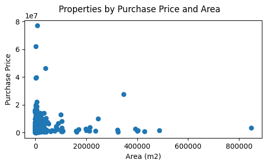
Let's look at a scatter plot of the data: property sales across NSW in the last six months (having an area >= 1):

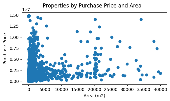
I very obviously have a few outliers! So let's see what it looks like when I filter on area <= 40,000 and price <= 15,000,000:

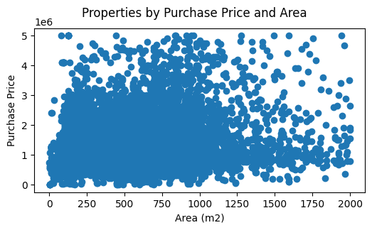
A bit better, but still it's clear there is a huge cluster at the low-end and sparse data at the high-end. I'll do one further refinement:

This looks a bit better, with less than 5% of the dataset removed. Now it's ready for use in a model.
Step 2: Using a machine learning model.
I've been learning using scikit-learn, an open source Python library. In scikit-learn, there are many different modules available for both regression and classification. Since a house price could theoretically be any number, I need to use a regression model. If I wanted to choose whether a property was a house or a unit based on certain features (i.e. a finite/pre-determined set of results), I'd use a classification model. For this particular problem, I've chosen Decision Tree regression for the following reasons:
- I have a small number of features;
- The data is very noisy and does not include a lot of variables which correlate with property prices (e.g. new/old house/apartment, views, etc.);
- I can validate the model fairly easily (this will be explored later).
There are downsides to decision trees, such as a risk of overfitting. Again, with this model just being for fun, I'll explore testing the accuracy of my model knowing that it is not completely accurate.
The code can be broken down into a few steps:
- Create the x and y datasets;
- Split the data into 'training' data and 'test' data sets ( train_test_split from scikit-learn can be used for this);
- Fit the training data to the model;
- Test the model against the test set;
- Validate the model.
This is a very, very simple example of the above steps (based on the scikit-learn documentation, not my actual code), and reading the data from csv into a pandas DataFrame:
import pandas as pd


from sklearn.tree import DecisionTreeRegressor


from sklearn.model_selection import train_test_split


# load the data into a dataframe


df = pd.read_csv('house_price_data.csv')


# create the x dataset using the features which will be used for prediction


features_x = df[['Postcode','Area','Type']]


# create the y dataset using the feature that will be predicted


features_y = df['PurchasePrice']


# split the dataset into a training set and a testing set


X_train, X_test, y_train, y_test = train_test_split(features_x, features_y, test_size=0.33, random_state=42)


# fit the data to the model


model = DecisionTreeRegressor()


model.fit(X_train, y_train)


# make predictions using the test set


y_predictions = model.predict(X_test)
After the model has been fit and applied to the test set, I can compare the predicted values against the actual values. Here are a few of those results:
| Actual | Predicted |
|---|---|
| 505,000 | 470,000 |
| 1,460,000 | 1,499,738 |
| 1,615,000 | 1,623,333 |
| 491,000 | 498,000 |
| 1,195,000 | 1,000,000 |
| 2,495,000 | 2,808,000 |
| 651,000 | 935,000 |
Some of these aren't too bad! But some predictions are way off, e.g. predicting 935,000 when the actual price was 651,000. As previously stated, there are many, many variables when it comes to property prices, and if I were to build a real model, I'd be looking to get additional data from multiple sources in order to improve the model.
Since I'm using train_test_split, this generates a random test data set each time I run the script. Another way I can check my results is by considering what tolerance there might be for incorrect predictions. Let's say that people would tolerate a prediction within $50,000 of the actual price (either positive or negative). I can create a dataframe which has a new column, "Difference", and calculate the difference between the actual result and the predicted result. When doing this, I regularly get about 45% of the results within $50k of the actual price.
Well, the model isn't accurate on the whole, but maybe it's more accurate for some suburbs than others? To test this, I can split my data into datasets by postcode, and then run the model. When I run this, I can look at the top 10 results:
| Postcode | Total Properties | Percent +/- 50k |
|---|---|---|
| 2216 | 310 | 84.47 |
| 2140 | 53 | 83.33 |
| 2760 | 80 | 81.48 |
| 2762 | 752 | 80.32 |
| 2147 | 191 | 75.00 |
| 2170 | 540 | 72.63 |
| 2530 | 84 | 71.43 |
| 2161 | 91 | 70.97 |
| 2192 | 49 | 70.59 |
| 2529 | 60 | 70.00 |
And the bottom 10 results:
| Postcode | Total Properties | Percent +/- 50k |
|---|---|---|
| 2207 | 27 | 0.00 |
| 2064 | 24 | 0.00 |
| 2119 | 58 | 5.00 |
| 2508 | 50 | 5.88 |
| 2226 | 40 | 7.14 |
| 2072 | 34 | 8.33 |
| 2516 | 35 | 8.33 |
| 2222 | 25 | 11.11 |
| 2334 | 23 | 12.50 |
| 2117 | 46 | 12.50 |
When viewing the results from this perspective, the model is reasonably accurate for some suburbs, but very inaccurate for other suburbs. This is a clear indicator that more data is required, as there might be external influences in some suburbs that are not being accounted for in my current data set.
To further demonstrate why more data is required, let's compare this result with a dataset which is more predictable. I've taken the Ausgrid Solar Home Electricity Data from 2012-2013 and created a very simple regression model to compare against. This data contains the kWh Gross Generation (GG) of solar energy, General Consumption for electricity supplied (GC), and Controlled Load Consumption (CL) for an anonymised subset of customers at 30 minute intervals (see the documentation for further details).
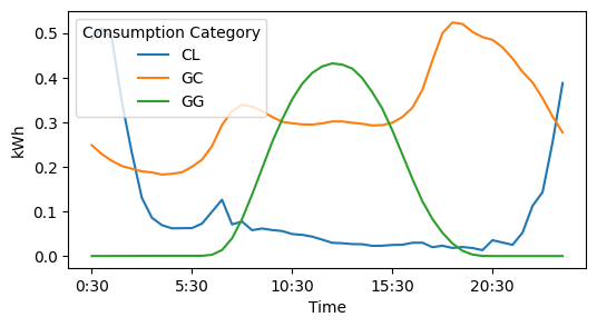
Again, first explore the data. I've taken the mean of kWh by consumption category for every half hour interval and charted it below:

All three points trend differently with time of day. Solar Gross Generation (GG) increases with time of day, then decreases after noon (which would correspond with the movement of the sun). Average General Consumption (GC) changes with time of day as well, peaking in the evenings. And Controlled Load Consumption (CL) relates to off-peak usage (refer to the Ausgrid documentation for further clarification). So what happens if I create a model which tries to predict solar energy generated (Consumption Category = GG) at 12pm based on the generation at other times of the day? Here are some results from testing that model (this time using a more simple linear regression model, not a decision tree):
| Actual | Predicted |
|---|---|
| 0.649 | 0.63725218 |
| 0.26 | 0.19205626 |
| 0.381 | 0.37382028 |
| 0.281 | 0.34235388 |
| 0.713 | 0.70965843 |
| 0.15 | 0.15955266 |
| 0.375 | 0.35789408 |
| 0.263 | 0.26636166 |
Not bad, but a couple of points are a bit off. In the property prices data set, I assumed that a prediction plus or minus $50k of the actual result would be tolerated, but with kWh being a much smaller scale I can't make the same assumption. I can, however, validate the overall results with a few regression metrics:
from sklearn.metrics import mean_squared_error, r2_score, mean_absolute_error


print('Mean Absolute Error: ', mean_absolute_error(y_test, y_pred))


print('Mean Squared Error: ', mean_squared_error(y_test, y_pred))


print('R2: ', r2_score(y_test, y_pred))
Mean Absolute Error:  0.04389801370636383


Mean Squared Error:  0.006005026143648444


R2:  0.9550457939927733
The Mean Absolute Error is the average of all errors, the Mean Squared Error represents the total amount of error in the results (smaller is better), and the R2 value calculates how well the model fits the data (closer to 1 is better). This model with multiple variables appears to be much better at prediction than the property price model. Turns out, solar electricity generation is much more predictable than property prices. Who'd have thought?
References and data sources:
- NSW property sales data sourced from NSW Valuer General.
- Ausgrid Solar Home Electricity Data sourced from Ausgrid.
- Machine learning models use scikit-learn.
- Other Python libraries in use include pandas and Matplotlib.
Data used in accordance with Creative Commons Attribution 4.0 International License.