Predictive modelling on the IMDb Dataset

In my previous blog post I used descriptive analytics on the IMDb dataset of movies to find the most popular genres across the 500 top movies of the last 50 years.

This analysis showed a peak in "top" movies around 2014, and then a decline even though the quantity of movies being released was increasing.

For the next task on this dataset, I wanted to see if I could build a classification model which could predict whether a movie would be popular or not.

To start, I had to decide what a "top" movie looked like, or what features defined a popular movie. I decided to focus on the top 5% of movies (based on weighted votes) released between 2007 and 2017. This is a different definition of a top movie from my previous analysis for the following reasons:

• Tastes in movies change over time, so comparing top movies over more than 10 years may not give accurate results;
• The dataset would have been very large to process with a classification model, and I am limited by compute capacity;
• The dataset would have been very imbalanced, which is more challenging to classify.

While the second and third points are more about feasibility, the first point is about the outcome. If I were to use movies from 1975 to predict whether a movie released in 2022 would be popular or not, it's not exactly a like-for-like comparison. This is because some of the defining features of popular movies include:

• The genre(s);
• The director(s);
• The writer(s);
• The actor(s) (IMDb dataset contains the first 10 by casting order).

All of these are dependent on the era in which a movie is released.

I also chose to compare movies from the decade where the number of votes hit its peak (2014). This also avoided the period between 2019 and 2021 where COVID-19 caused a decline in both movies being released and the number of votes on movies released in those years on the IMDb website.

Another big caveat on this dataset is that the popularity of movies is voted on by the users of IMDb. The demographics of users are not available publicly, so I cannot comment on this, but the classification model will be learning based on the votes of a specific demographic (IMDb interactive users) as opposed to a randomised sample of the population.

Choosing a library

I decided to use XGBoost as it is a fast and popular library for machine learning problems. It is well documented and I can be sure it'll run efficiently on my computer (as long as I control my dataset and parameters as much as possible). I also know that I want a classification model because I want to predict a binary value (true or false) based on a number of features, and XGBoost is good for binary classification.

Data exploration and pre-processing

I had explored the data in my previous analysis, but now I had to prepare it for its new purpose in a predictive model. I performed the following:

• Removing any movies with 0 runtime minutes;
• Removing any records with unknown genre, 0 votes, and 0 rating;
• Selecting only records with the type "movie" (excluded "tvMovie");
• Selecting only movies released between 2007 and 2017;
• Creating the new binary target variable "top movie" based on whether the record had weighted votes in the top 5% of this population;
• Changing the runtime minutes to categories (e.g. under 60 minutes, between 60 and 90 minutes, etc.) instead of a numerical value to allow conversion to binary values.

This leaves me with a dataset which still contains tens of thousands of records. With only 5% being classified as a top movie, this is a very imbalanced dataset which needs to be managed in my model.

Next is feature engineering, or transforming the data into features that will be more useful with a classification model. This isn't difficult for features like the genres, because there are only 25 unique genres which means I can convert this to 25 binary (true/false) columns. But what does it mean for the actors, directors, and writers?

In the dataset, there are:

• Around 300,000 unique actors;
• Around 50,000 unique directors;
• Around 80,000 unique writers.

To convert every unique person into a binary column would be both inefficient and unnecessary. To manage this, I trimmed the values down to only the actors, directors, and writers who belong to top movies, and then I further removed anyone who was associated with fewer than 3 movies.

These changes result in my dataset looking like this:

• Over 68,000 records;
• Over 4,000 columns;
• Over 4,000 top movies.

Building the model

Because my dataset is imbalanced, there's a risk of any model favouring the majority class (that is, the non-top movies which are 95% of the dataset), so I am using scale_pos_weight to balance the positive and negative. I also use RandomizedSearchCV from scikit-learn to perform a randomised search to find good hyperparameters for the XGBoost model, targeting a good average precision score.

I also split my dataset into a training set (70% of the data) and a testing set (30% of the data), so I had separate sets to train the model and validate it.

Because XGBoost is efficient, it only takes a few minutes for the model to train based on the training set, and predict based on the testing set.

Evaluating the model

After all this work, how do I know whether this model is any good? Fortunately there are several ways to evaluate a model.

Confusion matrix

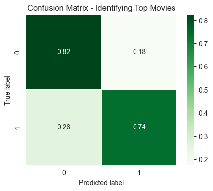
The confusion matrix identifies how well my model predicted values in the test set. In this case, the model correctly predicted 74% of the top movies as top movies (true/1), but it misclassified 26% as false or 0. It also misclassified 18% of non-top movies as being popular movies (i.e. my model predicted true for the record, but the real value was false).

This isn't a bad result, but it's based on what the cost would be of getting a prediction wrong. If I recommended a movie which turned out to not be good, it could lead to mistrust. Alternatively, if I said "this movie isn't good", but it was actually one of the top 5% movies of the decade, then it's a missed opportunity.

Fortunately, neither of these misses are very important in my use case, but it matters for real world scenarios like medical diagnoses or fraud detection.

Precision-Recall Curve and Average Precision

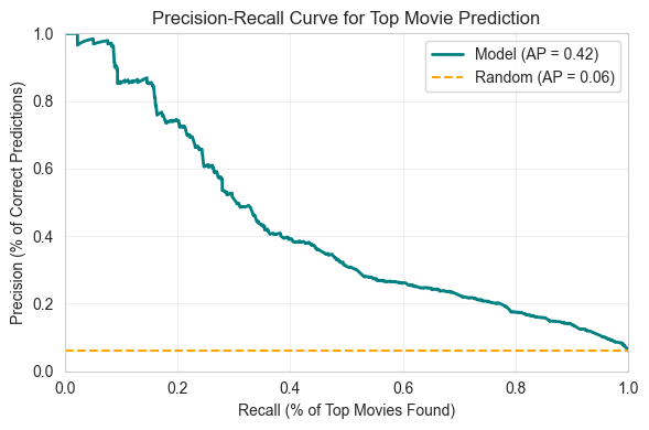
Precision describes the percentage of correctly identified top movies, and recall describes the percentage of all actual top movies found. A high precision means few false positives, and a high recall means few false negatives.

In the case of my model, it has an average precision/area under PR curve of 0.42, where random guessing is around 0.06 (the ratio of true values in the test dataset). So my model is about 7 times better than a random guess. Based on the complexity of the use case, this isn't a bad result.

Exploring top features

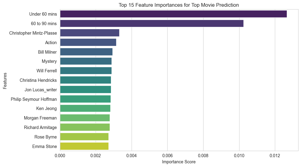
We can investigate which features contributed to the predictions. The above graph shows the importance the model put on each feature, from top to bottom (limited to the top 15 features). Importance doesn't necessarily mean a positive impact, though, so let's further explore correlation to see how these features correlated to the top movie indicator.

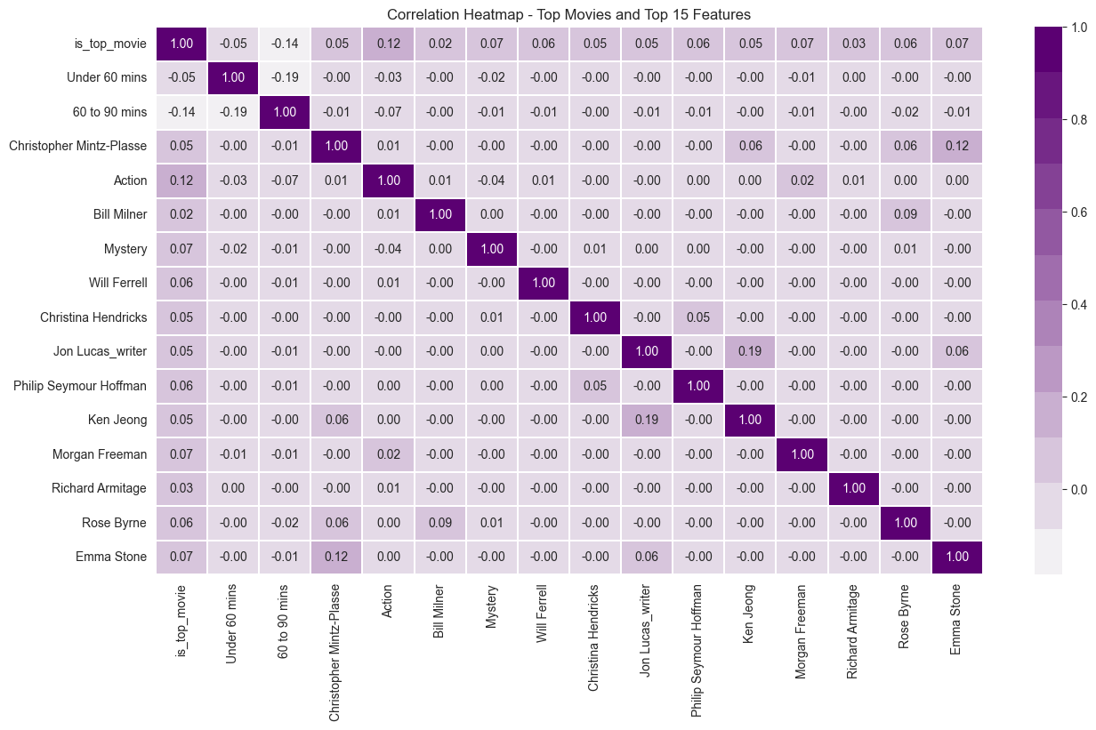
Even though a runtime of less than 60 minutes has a high importance, it has a negative correlation to the top movie prediction, which means movies under 60 minutes long are unlikely to be in the top 5%. Similarly, 60 to 90 minutes also has a negative correlation. However, all named actors/directors/writers in the top 15 features have a positive correlation.

It is also interesting to see positive correlations between actors/directors/writers, for example, Emma Stone and Christopher Mintz-Plasse, Kristen Bell and Jon Lucas, and Christina Hendricks and Philip Seymour Hoffman. Some actors, such as Will Ferrell and Morgan Freeman, have low/no correlation with other actors.

In terms of genres, Action and Mystery each have a positive correlation with the top movie indicator, but a slightly negative correlation with each other. This means you're unlikely to see a top movie which is both Action and Mystery (more likely Action/Adventure and Mystery/Horror).

We can see the split of top movies by their runtime in a bar chart:

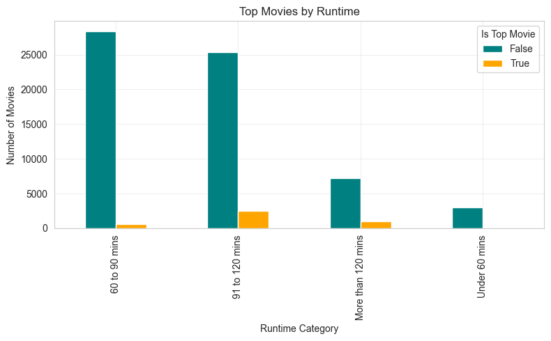
With this graph it's easy to see that movies which are more than 90 minutes runtime have a higher proportion of top movies than other categories, which is why the lower runtimes are important features with negative correlations.

Ultimately, it's difficult to predict whether a movie would be popular or not based on only this information. Even if a movie has a great cast, a fantastic director, creative writers, and in-demand genres, there's no guarantee that it would be popular. Still, it is a fun dataset to explore, and building a classification model on a complex dataset was a great learning experience.

Information courtesy of IMDb (https://www.imdb.com). Used with permission.